Machine learning is a fascinating field of study which is growing at an extreme rate. As computers get faster and faster, we attempt to harness the power of these machines to tackle difficult, complex, and/or unintuitive problems in biology, mathematics, engineering, and physics. Many of the purely mathematical models used in these fields are extremely simplified compared to their real-world counter parts (see the spherical cow). As scientists attempt more and more accurate simulations of our universe, machine learning techniques have become critical to building accurate models and estimating experimental parameters.
Also, even very basic machine learning can be used to effectively block spam email, which puts it somewhere between water and food on the "necessary for life" scale.
BAYES FORMULA - GREAT FOR GROWING BODIES
Machine learning seems very complicated, and advanced methods in the field are usually very math heavy - but it is all based in common statistics, mostly centered around the ever useful Gaussian distribution. One can see the full derivation for the below formulas here (PDF) or here (PDF), a lot of math is involved but it is relatively straightforward as long as you remember Bayes rule:
$posterior \:=\: likelihood \:\times\: prior$
HE DIDN'T MEAN IT
From the links above, we can see that our best estimate for the mean $\mu$ given a known variance $\sigma^2$ and some Gaussian distributed data vector $X$ is:
$\sigma(\mu)^2_n = {\Large \frac{1}{\frac{N}{\sigma^2}+\frac{1}{\sigma_o^2}}}$
$\mu_n = {\Large \frac{1}{\frac{N}{\sigma^2}+\frac{1}{\sigma^2}}(\frac{\sum\limits_{n=1}^N x_n}{\sigma^2}+\frac{\mu_o}{\sigma_o^2})}$
where $N$ (typically 1) represents the number of $X$ values used to generate the mean estimate $\mu$ (just $x_n$ if $N$ is 1), $\mu_o$ is the previous "best guess" for the mean ($\mu_{n-1}$), $\sigma_o^2$ is the previous confidence in the "best guess" for $\mu$ ($\sigma(\mu)^2_{n-1})$), and $\sigma$ was known prior to the calculation. Lets see what this looks like in python.
#!/usr/bin/python
import numpy as np
import matplotlib.pyplot as plot
total_obs = 1000
primary_mean = 5.
primary_var = known_var = 4.
x = np.sqrt(primary_var)*np.random.randn(total_obs) + primary_mean
f, axarr = plot.subplots(3)
f.suptitle("Unknown mean ($\$$\mu=$\$$"+`primary_mean`+"), known variance ($\$$\sigma^2=$\$$"+`known_var`+")")
y0label = "Timeseries"
y1label = "Estimate for mean"
y2label = "Doubt in estimate"
axarr[0].set_ylabel(y0label)
axarr[1].set_ylabel(y1label)
axarr[2].set_ylabel(y2label)
axarr[0].plot(x)
prior_mean = 0.
prior_var = 1000000000000.
all_mean_guess = []
all_mean_doubt = []
for i in range(total_obs):
posterior_mean_doubt = 1./(1./known_var+1./prior_var)
posterior_mean_guess = (prior_mean/prior_var+x[i]/known_var)*posterior_mean_doubt
all_mean_guess.append(posterior_mean_guess)
all_mean_doubt.append(posterior_mean_doubt)
prior_mean=posterior_mean_guess
prior_var=posterior_mean_doubt
axarr[1].plot(all_mean_guess)
axarr[2].plot(all_mean_doubt)
plot.show()
This code results in this plot:
 We can see that there are two basic steps - generating the test data, and iteratively estimating the "unknown parameter", in this case the mean. We begin our estimate for the mean at any value (prior_mean = 0) and set the prior_var variable extremely large, indicating that our confidence in the mean actually being 0 is extremely low.
V FOR VARIANCE
What happens in the opposite (though still "academic" case) where we know the mean but not the variance? Our best estimate for unknown variance $\sigma^2$ given the mean $\mu$ and some Gaussian distributed data vector $X$ will use some extra variables, but still represent our estimation process.:

INTO THE UNKNOWN(S)#!/usr/bin/python
import numpy as np
import matplotlib.pyplot as plot
total_obs = 1000
primary_mean = 5.
primary_var = known_var = 4.
x = np.sqrt(primary_var)*np.random.randn(total_obs) + primary_mean
f, axarr = plot.subplots(3)
f.suptitle("Unknown mean ($\$$\mu=$\$$"+`primary_mean`+"), known variance ($\$$\sigma^2=$\$$"+`known_var`+")")
y0label = "Timeseries"
y1label = "Estimate for mean"
y2label = "Doubt in estimate"
axarr[0].set_ylabel(y0label)
axarr[1].set_ylabel(y1label)
axarr[2].set_ylabel(y2label)
axarr[0].plot(x)
prior_mean = 0.
prior_var = 1000000000000.
all_mean_guess = []
all_mean_doubt = []
for i in range(total_obs):
posterior_mean_doubt = 1./(1./known_var+1./prior_var)
posterior_mean_guess = (prior_mean/prior_var+x[i]/known_var)*posterior_mean_doubt
all_mean_guess.append(posterior_mean_guess)
all_mean_doubt.append(posterior_mean_doubt)
prior_mean=posterior_mean_guess
prior_var=posterior_mean_doubt
axarr[1].plot(all_mean_guess)
axarr[2].plot(all_mean_doubt)
plot.show()
This code results in this plot:

V FOR VARIANCE
What happens in the opposite (though still "academic" case) where we know the mean but not the variance? Our best estimate for unknown variance $\sigma^2$ given the mean $\mu$ and some Gaussian distributed data vector $X$ will use some extra variables, but still represent our estimation process.:
$a_n = {\Large a_o + \frac{N}{2}}$
$b_n = {\Large b_o + \frac{1}{2}\sum\limits^N_{n=1}(x_n-\mu)^2}$
$\lambda = {\Large \frac{a_n}{b_n}}$
$\sigma(\lambda)^2 = {\Large \frac{a_n}{b_n^2}}$
where
$\lambda = {\Large \frac{1}{\sigma^2}}$
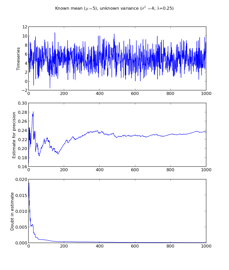
This derivation is made much simpler by introducing the concept of precision ($\lambda$), which is simply 1 over the variance. We estimate the precision, which can be converted back to variance if we prefer. $\mu$ is known in this case.
#!/usr/bin/python
import numpy as np
import matplotlib.pyplot as plot
total_obs = 1000
primary_mean = known_mean = 5
primary_var = 4
x = np.sqrt(primary_var)*np.random.randn(total_obs) + primary_mean
all_a = []
all_b = []
all_prec_guess = []
all_prec_doubt = []
prior_a=1/2.+1
prior_b=1/2.*np.sum((x[0]-primary_mean)**2)
f,axarr = plot.subplots(3)
f.suptitle("Known mean ($\$$\mu=$\$$"+`known_mean`+"), unknown variance ($\$$\sigma^2=$\$$"+`primary_var`+"; $\$$\lambda$\$$="+`1./primary_var`+")")
y0label = "Timeseries"
y1label = "Estimate for precision"
y2label = "Doubt in estimate"
axarr[0].set_ylabel(y0label)
axarr[1].set_ylabel(y1label)
axarr[2].set_ylabel(y2label)
axarr[0].plot(x)
for i in range(1,total_obs):
posterior_a=prior_a+1/2.
posterior_b=prior_b+1/2.*np.sum((x[i]-known_mean)**2)
all_a.append(posterior_a)
all_b.append(posterior_b)
all_prec_guess.append(posterior_a/posterior_b)
all_prec_doubt.append(posterior_a/(posterior_b**2))
prior_a=posterior_a
prior_b=posterior_b
axarr[1].plot(all_prec_guess)
axarr[2].plot(all_prec_doubt)
plot.show()
Here I chose to set the values for prior_a and prior_b to the "first" values of the estimation, we could just as easily have reversed the formulas by setting the precision to some value, and the "doubt" about that precision very large, then solving a system of two equations, two unknowns for a and b.
What happens if both values are unknown? All we really know is that the data is Gaussian distributed!
$\nu_o={\Large \kappa_o-1}$
$\mu_n={\Large \frac{\kappa_o\mu_o+\overline{X}N}{\kappa_o+N}}$
$\kappa_n={\Large \kappa_o+N}$
$\nu_n={\Large \nu_o+N}$
$\sigma_n^2={\Large \frac{\nu_o\sigma^2+(N-1)s^2+\frac{\kappa_oN}{\kappa_o+N}(\overline{X}-\mu_o)^2}{\nu_n}}$
$s={\Large var(X)}$
The technique here is the same as other derivations for unknown mean, known variance and known mean, unknown variance. To estimate the mean and variance of data taken from a single Gaussian distribution, we need to iteratively update our best guesses for both mean and variance. In many cases, $N=1$, so the value for $s$ is not necessary and $\overline{X}$ becomes $x_n$. Let's look at the code.
#!/usr/bin/python
import matplotlib.pyplot as plot
import numpy as np
total_obs = 1000
primary_mean = 5.
primary_var = 4.
x = np.sqrt(primary_var)*np.random.randn(total_obs) + primary_mean
f, axarr = plot.subplots(3)
f.suptitle("Unknown mean ($\$$\mu=$\$$"+`primary_mean`+"), unknown variance ($\$$\sigma^2=$\$$"+`primary_var`+")")
y0label = "Timeseries"
y1label = "Estimate for mean"
y2label = "Estimate for variance"
axarr[0].set_ylabel(y0label)
axarr[1].set_ylabel(y1label)
axarr[2].set_ylabel(y2label)
axarr[0].plot(x)
prior_mean = 0.
prior_var = 1.
prior_kappa = 1.
prior_v = 0.
all_mean_guess = []
all_var_guess = []
for i in range(total_obs):
posterior_mean = (prior_kappa*prior_mean+x[i])/(prior_kappa + 1)
posterior_var = (prior_v*prior_var + prior_kappa/(prior_kappa + 1)*(x[i]-prior_mean)**2)/(prior_v + 1)
prior_kappa += 1
prior_v += 1
all_mean_guess.append(posterior_mean)
all_var_guess.append(posterior_var)
prior_mean = posterior_mean
prior_var = posterior_var
axarr[1].plot(all_mean_guess)
axarr[2].plot(all_var_guess)
plot.show()

SOURCES
Pattern Recognition and Machine Learning, C. Bishop
Bayesian Data Analysis, A. Gelman, J. Carlin, H. Stern, and D. Rubin
Classnotes from Advanced Topics in Pattern Recognition, UTSA, Dr. Zhang, Spring 2013
Is there a reason why, in the first example (known variance, unknown mean), the "doubt" is so much lower than the error in the estimate, for the first several hundred samples?
ReplyDeleteFor example, after 200 samples, the "doubt" is well below 0.1, but the estimate of the mean is still wrong by about 0.1. It seems that your "doubt" figure is much too optimisitic.
If you're presenting these figures to somebody who doesn't want a ton of explanation (like maybe your manager at work) it would probably be better to use the standard deviation, or even better a 95% confidence interval, instead of your "doubt" value.
The variable I labeled "doubt" is the variance of precision in statistics lingo ($/frac{1}{\sigma^2}$). I chose a different label because I felt it was a simpler, more general term to describe what that parameter really means, especially to people less familiar with statistics terminology.
DeleteThe tricky part about "doubt" is that because it is a variance, it suffers a serious problem - namely that something can have a very low deviation, doubt, or variance, and still have an incorrect (or biased) result. That is what you see in the second example - the algorithm converged on a given solution based on the data we input, but we know that answer is incorrect, since we are lucky enough to know "ground truth". Maybe given more samples we would eventually have arrived at the true answer (looking at the upward trend in the estimate), but all we have to go by right now are these 1000 samples.
This is a problem in nearly every scientific field - how do we validate our results and eliminate possible bias, when we have no idea what "ground truth" actually is? And specifically for machine learning - how do we validate the results of algorithms on our datasets, when the volume of data eliminates classic "check by hand" approaches, and we are using these approaches in an exploratory fashion i.e. we have no conception of what the answers should be?
I really, really like your idea about using the 95% confidence interval. I think it is is a superior approach to what I am doing now - the same information can be displayed in two graphs instead of three. I will definitely look into that! Thanks for your comments
Edit: the formula above should be $\frac{1}{\sigma^2}$
DeleteIs there seriously no way to edit comments?
Machine Learning Training in Hyderabad at AI Patasala will allow you to maximize the subject knowledge of your candidates. Aspirants will be able to get a certification in Machine Learning at AI Patasala, which will allow them to create the best career path.
ReplyDeleteMachine Learning Course with Placements in Hyderabad