Continuing our exploration of machine learning, we will discuss the use of basis functions for regression analysis. When presented with an unknown dataset, it is very common to attempt to find trends or patterns. The most basic form of this is visual inspection - how is the data trending? Does it repeat in cycles? Can we predict future data given some past events? The mathematical approach to this "trend finding" is called regression, or line fitting. As we will see, it is possible to fit more than a simple straight line, and the general technique of regression is very effective at breaking down many types of data.
DRY DRY DERIVATION
What are some sample functions we might want to perform regression on? Take as an example:
$y = x^2 - 4x + 1$

What happens if we look at the same values, distorted by some noise?

Since we know the original function for the data, it is easy to "see" the underlying $x^2 - 4x +1$ (the blue line) is still there, but how can we do this mathematically, and without knowledge of the original generating function?
If we think of any $n$th order polynomial, $y({\bf w}, {\bf x})$, it can always be represented by the form.
$y({\bf w}, {\bf x}) = w_0 + w_1x_1 + w_2x_2+\ldots + w_nx_n$
This can also be represented in matrix form.
$[w_0\ldots w_{n}]\left[ \begin{array}{xmat} 1 & 0 & \cdots & 0\\ 0 & x_1 & \cdots & 0 \\ \vdots & \vdots & \ddots & \vdots \\ 0 & 0 & \cdots & x_n \end{array} \right]$
BASE CAMP 1KM
In fact, going one step further, we see that the vector ${\bf x}$ could really be better generalized as a basis vector - that is, our current vector ${\bf x} = [0, x, x^2] = x^n$ could be generalized with something besides $x^n$. We could use sine waves (Fourier basis), Gaussians, sigmoids, wavelets, or any number of other functions to perform this same regression - in fact, this is the root of the concept of transforms in DSP lingo.
When we talk about linear regression, we are really talking about a linear regression in the basis domain - a linear combination of basis functions multiplied by weighting values, which can be used to approximate the original signal. Since we have learned that we can use nearly any function as a basis, let's change notation from ${\bf x}$ to ${\bf \phi}$, where ${\bf \phi}$ is a function of $x$.
$[w_o\ldots w_{n}]\left[ \begin{array}{phimat} \phi_0(x_1) & \phi_0(x_2) & \cdots
& \phi_0(x_n) \\ \phi_1(x_1) & \phi_1(x_2) & \cdots & \phi_1(x_n) \\ \vdots & \vdots
& \ddots & \vdots \\ \phi_m(x_1) & \phi_m(x_2) & \cdots & \phi_m(x_n)
\end{array} \right]$
The full derivation of the maximum likelihood estimate (MLE) can be found here, but the short and sweet version is that the maximum likelihood estimate of ${\bf w}$ is $(\Phi^T\Phi)^{-1}\Phi {\bf t}$, where $\Phi$ is the general basis matrix defined above, and ${\bf t}$ is a set of test datapoints. These test datapoints are generated by $\Phi {\bf w_m}$, where ${\bf w_m}$ are the measured values (red dots shown in the above figures).
$(\Phi^T\Phi)^{-1}\Phi$ is known as the Moore-Penrose pseudoinverse, and it can be replaced by the matrix inverse $\Phi^{-1}$ if the basis matrix is square (3x3, 100x100, etc.). Let's look at the code.
$(\Phi^T\Phi)^{-1}\Phi$ is known as the Moore-Penrose pseudoinverse, and it can be replaced by the matrix inverse $\Phi^{-1}$ if the basis matrix is square (3x3, 100x100, etc.). Let's look at the code.
#!/usr/bin/python
import numpy as np
import matplotlib.pyplot as plot
import math
def gen_dft(m, n, N):
return np.exp(1j*-2*m*n/N)
def gen_polynomial(x, m):
return x**m
N = 10
N_basis = 3
noise_var = B = 5
basis = np.matrix(np.zeros((N,N)), dtype=np.complex64)
xs = np.matrix(range(N)).T
ys = np.square(xs) - 4*xs + 1
wm = ys + np.sqrt(B)*np.random.randn(N,1)
for m in range(N_basis):
for n in range(N):
if m == 0:
basis[m,n] = 1.0
else:
basis[m,n] = gen_polynomial(xs[n], m)
#To use the gen_dft basis, make sure to set N_basis = N
#basis[m,n] = gen_dft(m, n, N)
test_data = t = basis*wm
#Calculate using the Moore-Penrose pseudoinverse using the following formula
#maximum_likelihood = wml = np.linalg.inv(basis.T*basis)*basis.T*t
#Direct calculation appears to have numerical instability issues...
#Luckily the pinv method calculates Moore-Penrose pseudo inverse using SVD
#which largely avoids the numerical issues
maximum_likelihood = wml = np.linalg.pinv(basis)*t
plot.figure()
plot.title("Regression fit using polynomial basis function, number of basis functions = $\$$" + `N_basis` + "$\$$")
plot.plot(ys, 'b')
plot.plot(wm, 'ro')
plot.plot(np.real(wml), 'g')
plot.show()
As we can see, the approximation with 3 basis functions (2nd order polynomial fit) does a pretty good job of approximating the original function. Let's see what happens if we increase the number of basis functions.


We can see that this fit gets closer to the measured data (red dots), but is actually further from the true signal without noise! This is called overfitting, because our estimate is beginning to fit our measurement, which has noise, rather than the underlying function (the blue line). Let's try another example, using the Fourier basis matrix.
The Fourier basis does a decent job of fitting the line, but still has more error than the polynomial fit with the right number of basis functions. Because the original function is polynomial, we should expect a polynomial basis to give superior results. We are overfitting our polynomial regression by including too many basis functions - in general, we want to fit the smallest number of basis functions while still minimizing overall error.

BAYES ASPIRIN
So how do we actually perform a Bayesian regression? There are some complicated derivations once again (pg 17 and onward here), but the idea is that we make iterative estimates, starting with some prior estimate and a likelihood to get a posterior estimate, which we will use as the prior for the next iteration. Remember, Bayesian is all about $posterior\: =\: likelihood\: \times\: prior$. After iterating through all the data points, we expect our estimate to approach the true generating function, without noise. Let's look at the code.
#!/usr/bin/python
import numpy as np
import matplotlib.pyplot as plot
N = 10
noise_var = B = .2**2
lower_bound = lb = 0.
upper_bound = ub = 5.
xs = np.matrix((ub-lb)*np.random.rand(N)+lb).T
xaxis = np.matrix(np.linspace(lb,ub,num=N)).T
w = np.array([1, -4, 1])
ys = w[0] + w[1]*xaxis + w[2]*np.square(xaxis)
t = w[0] + w[1]*xs + +w[2]*np.square(xs) + np.sqrt(B)*np.random.randn(N,1);
def gen_polynomial(x, p):
return x**p
N_basis = 7
alpha = a = 1.
beta = b = 1./B;
prior_m = np.zeros((N_basis, 1))
m = np.zeros((N_basis, N))
prior_s = np.matrix(np.diag(np.array([a]*N_basis)))
s = np.zeros((N_basis, N_basis))
plot.figure()
for n in range(N):
poly = np.vectorize(gen_polynomial)
basis = poly(xs[n], np.matrix(np.arange(N_basis)))
s_inv = prior_s.I*np.eye(N_basis)+b*(basis.T*basis)
s = s_inv.I*np.eye(N_basis)
#Need to use .squeeze() so broadcasting works correctly
m[:,n] = (s*(prior_s.I*prior_m+(b*basis.T*t[n]))).squeeze()
y = m[0,n] + m[1,n]*xaxis + m[2,n]*np.square(xaxis)
plot.plot(xaxis, y, "g")
prior_m[:,0] = m[:,n].squeeze()
prior_s = s
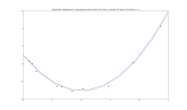
plot.title("Bayesian regression using polynomial basis function, number of basis functions = $\$$" + `N_basis` + "$\$$")
plot.plot(xaxis, ys, "b")
plot.plot(xs, t, "ro")
plot.plot(xaxis, y, "k")
plot.show()
 Adding in the progression plots (plot.plot(xaxis, y, "g"))
 The green lines show how the Bayesian regression updates on each iteration through the loop - though unlabeled, we assume that the closer the green line is to the final estimate (black line), the later it ran in the code, with the n = 10 iteration resulting in the final black line shown.
The top part of the code sets up the generating function, also generates samples corrupted by noise. We could set xs differently to get linearly spaced samples (using np.arange(lb,ub,N)) instead of random spacing, but random samples are what Bishop is using in his book and diagrams (Pattern Recognition and Machine Learning, C. Bishop). I also chose to vectorize the basis matrix generation this time - which doesn't actually increase the code speed (in numpy at least), but does turn a multi-line for loop into one line of code.
In fact, looking at page 153 in Bishop's book will give all the formulas used in the processing loop, mapped as follows.

#!/usr/bin/python
import numpy as np
import matplotlib.pyplot as plot
N = 10
noise_var = B = .2**2
lower_bound = lb = 0.
upper_bound = ub = 5.
xs = np.matrix((ub-lb)*np.random.rand(N)+lb).T
xaxis = np.matrix(np.linspace(lb,ub,num=N)).T
w = np.array([1, -4, 1])
ys = w[0] + w[1]*xaxis + w[2]*np.square(xaxis)
t = w[0] + w[1]*xs + +w[2]*np.square(xs) + np.sqrt(B)*np.random.randn(N,1);
def gen_polynomial(x, p):
return x**p
N_basis = 7
alpha = a = 1.
beta = b = 1./B;
prior_m = np.zeros((N_basis, 1))
m = np.zeros((N_basis, N))
prior_s = np.matrix(np.diag(np.array([a]*N_basis)))
s = np.zeros((N_basis, N_basis))
plot.figure()
for n in range(N):
poly = np.vectorize(gen_polynomial)
basis = poly(xs[n], np.matrix(np.arange(N_basis)))
s_inv = prior_s.I*np.eye(N_basis)+b*(basis.T*basis)
s = s_inv.I*np.eye(N_basis)
#Need to use .squeeze() so broadcasting works correctly
m[:,n] = (s*(prior_s.I*prior_m+(b*basis.T*t[n]))).squeeze()
y = m[0,n] + m[1,n]*xaxis + m[2,n]*np.square(xaxis)
plot.plot(xaxis, y, "g")
prior_m[:,0] = m[:,n].squeeze()
prior_s = s
plot.title("Bayesian regression using polynomial basis function, number of basis functions = $\$$" + `N_basis` + "$\$$")
plot.plot(xaxis, ys, "b")
plot.plot(xs, t, "ro")
plot.plot(xaxis, y, "k")
plot.show()


The top part of the code sets up the generating function, also generates samples corrupted by noise. We could set xs differently to get linearly spaced samples (using np.arange(lb,ub,N)) instead of random spacing, but random samples are what Bishop is using in his book and diagrams (Pattern Recognition and Machine Learning, C. Bishop). I also chose to vectorize the basis matrix generation this time - which doesn't actually increase the code speed (in numpy at least), but does turn a multi-line for loop into one line of code.
In fact, looking at page 153 in Bishop's book will give all the formulas used in the processing loop, mapped as follows.
s_inv = ${\bf S}_N^{-1}$
s = ${\bf S}_N$
m[:,n] = ${\bf m}_N$
prior_s = ${\bf S}_0^{-1}$
prior_m = ${\bf m}_0$
Updating the priors with the results of the loop each time, we end up with a reasonable approximation of the generating function as long as N_basis is the same as the generating function. What happens if we don't use the right value for N_basis?

Bad things, it turns out. Instead of an overfitting problem, we now have a model selection problem - if we don't choose N_basis right, we won't converge to the right answer!
AUTO MODELING AND DETAILING
We really want to automate this model selection process, as scientists are too busy traveling the world and winning awards to babysit their award-winning scientific models. Luckily, there is a formula for calculating Bayesian model evidence - the model that maximizes this function should be the best choice! See the notes here (PDF) for more details, starting with slide 41.
${\large {\bf A} = {\bf S}_N^{-1} = \alpha {\bf I} + \beta {\bf \Phi}^T{\bf \Phi}}$
${\large {\bf m}_N = \beta{\bf A}^{-1}{\bf \Phi}^T{\bf t}}$
${\large E({\bf m}_N) = \frac{\beta}{2}||{\bf t}-{\bf \Phi}{\bf m}_N||^2+\frac{\alpha}{2}{\bf m}_N^T{\bf m}_N}$
${\large \ln p({\bf t}| \alpha, \beta) = \frac{M}{2}ln(\alpha)+\frac{N}{2}ln(\beta)-E({\bf m}_N) - \frac{1}{2}ln(| {\bf A} | ) - \frac{N}{2}ln(2\pi)}$
Approximations for $\alpha$ and $\beta$ are:

Approximations for $\alpha$ and $\beta$ are:
${\large \alpha = \frac{M}{2E_w({\bf m}_N)} = \frac{M}{{\bf w}^T{\bf w}}}$
${\large \beta = \frac{N}{2E_D({\bf m}_N)} = \frac{N}{\sum\limits^N_{n=1}\{t_n - {\bf w}^T\phi({\bf x}_n)\}^2}}$
By running each model, then computing the last equation (the model evidence function), we can see which model has the highest evidence of being correct. The full code for this calculation is listed below.
#!/usr/bin/python
import numpy as np
import matplotlib.pyplot as plot
N = 50.
noise_var = B = .2**2
lower_bound = lb = -5.
upper_bound = ub = 5.
xs = np.matrix(sorted((ub-lb)*np.random.rand(N)+lb)).T
xaxis = np.matrix(np.linspace(lb,ub,num=N)).T
w = np.array([1, -4, 1])
ys = w[0] + w[1]*xaxis + w[2]*np.square(xaxis)
t = w[0] + w[1]*xs + +w[2]*np.square(xs) + np.sqrt(B)*np.random.randn(N,1);
prior_alpha = 0.005 #Low precision initially
prior_beta = 0.005 #Low guess for noise var
max_N = 7 #Upper limit on model order
evidence = E = np.zeros(max_N)
f, axarr = plot.subplots(3)
def gen_polynomial(x, p):
return x**p
itr_upper_bound = 250
all_y = []
for order in range(1, max_N+1):
m = np.zeros((order, 1))
s = np.zeros((order, order))
poly = np.vectorize(gen_polynomial)
basis = poly(xs, np.tile(np.arange(order), N).reshape(N, order))
alpha = a = prior_alpha
beta = b = prior_beta
itr = 0
while not itr < itr_upper_bound:
itr += 1
first_part = a*np.eye(order)
second_part = b*(basis.T*basis)
s_inv = a*np.eye(order)+b*(basis.T*basis)
m = b*s_inv.I*basis.T*t
posterior_alpha = pa = np.matrix(order/(m.T*m))[0,0]
posterior_beta = pb = np.matrix(N/((t.T-m.T*basis.T)*(t.T-m.T*basis.T).T))[0,0]
a = pa
b = pb
A = a*np.eye(order)+b*(basis.T)*basis
mn = b*(A.I*(basis.T*t))
penalty = emn = b/2.*(t.T-mn.T*basis.T)*(t.T-mn.T*basis.T).T+a/2.*mn.T*mn
E[order-1] = order/2.*np.log(a)+N/2.*np.log(b)-emn-1./(2*np.log(np.linalg.det(A)))-N/2.*np.log(2*np.pi)
y = (mn.T*basis.T).T
all_y.append(y)
axarr[0].plot(xs, y ,"g")
best_model = np.ma.argmax(E)
#print E
x0label = x2label = "Input X"
y0label = y2label = "Output Y"
x1label = "Model Order"
y1label = "Score"
plot.tight_layout()
axarr[0].set_xlabel(x0label)
axarr[0].set_ylabel(y0label)
axarr[1].set_xlabel(x1label)
axarr[1].set_ylabel(y1label)
axarr[2].set_xlabel(x2label)
axarr[2].set_ylabel(y2label)
axarr[0].set_title("Bayesian model estimation using polynomial basis functions")
axarr[0].plot(xaxis, ys, "b")
axarr[0].plot(xs, t, "ro")
axarr[1].set_title("Model Evidence")
axarr[1].plot(E, "b")
axarr[2].set_title("Best model, polynomial order $"+`best_model`+"$")
axarr[2].plot(xs, t, "ro")
axarr[2].plot(xs, all_y[best_model], "g")
plot.show()

The model selection calculation has allowed us to evaluate different models and compare them mathematically. The model evidence values for this run are:
Let's add more noise and see what happens.

[-200.40318142 -187.76494065 -186.72241097 -189.13724168 -191.74123924 -194.37069482 -197.01120722]
Let's add more noise and see what happens.

Adjusting the noise_var value from .2**2 to 1.**2, we see that that the higher order models have increased bias, just as we saw in our earlier experiments. Our model evidence coefficients are:
This time, we are able to use the model evidence function to correctly compensate for model bias and select the best model for our data. Awesome! Let's push a little farther, and reduce the number of sample points as well.

We can see that with a reduced number of samples (N = 10), there is not enough information to accurately fit or estimate the model order. Our coefficients for this run were:
This is important point - all of these techniques help determine a model which is best for your data, but if there are not enough data points, or the data points are not unique enough to make a good assessment, you will not be able to get a grasp of the underlying function, which will lead to an imprecise answer. In the next installment of this series, we will cover another method of linear regression, which is easily extended to simplistic classification.
[-207.27716138 -195.14402961 -188.44030008 -190.92931379 -193.53242997 -196.16271701 -198.75960682]

[-46.65574626 -42.33981333 -43.95725922 -46.19200103 -49.68466447 -51.98193588 -54.56531748]
This is important point - all of these techniques help determine a model which is best for your data, but if there are not enough data points, or the data points are not unique enough to make a good assessment, you will not be able to get a grasp of the underlying function, which will lead to an imprecise answer. In the next installment of this series, we will cover another method of linear regression, which is easily extended to simplistic classification.
SOURCES
Pattern Recognition and Machine Learning, C. Bishop
Bayesian Data Analysis, A. Gelman, J. Carlin, H. Stern, and D. Rubin
Classnotes from Advanced Topics in Pattern Recognition, UTSA, Dr. Zhang, Spring 2013
Pattern Recognition and Machine Learning, C. Bishop
Bayesian Data Analysis, A. Gelman, J. Carlin, H. Stern, and D. Rubin
Classnotes from Advanced Topics in Pattern Recognition, UTSA, Dr. Zhang, Spring 2013